3.3. 模型评估: 量化预测的质量
校验者: @飓风 @小瑶 @FAME @v 翻译者: @小瑶 @片刻 @那伊抹微笑
有 3 种不同的 API 用于评估模型预测的质量:
- Estimator score method(估计器得分的方法): Estimators(估计器)有一个
score(得分)方法,为其解决的问题提供了默认的 evaluation criterion (评估标准)。 在这个页面上没有相关讨论,但是在每个 estimator (估计器)的文档中会有相关的讨论。 - Scoring parameter(评分参数): Model-evaluation tools (模型评估工具)使用 cross-validation (如
model_selection.cross_val_score和model_selection.GridSearchCV) 依靠 internal scoring strategy (内部 scoring(得分) 策略)。这在 scoring 参数: 定义模型评估规则 部分讨论。 - Metric functions(指标函数):
metrics模块实现了针对特定目的评估预测误差的函数。这些指标在以下部分部分详细介绍 分类指标, 多标签排名指标, 回归指标 和 聚类指标 。
最后, 虚拟估计 用于获取随机预测的这些指标的基准值。
See also
对于 “pairwise(成对)” metrics(指标),samples(样本) 之间而不是 estimators (估计量)或者 predictions(预测值),请参阅 成对的矩阵, 类别和核函数 部分。
3.3.1. scoring 参数: 定义模型评估规则
Model selection (模型选择)和 evaluation (评估)使用工具,例如 model_selection.GridSearchCV 和 model_selection.cross_val_score ,采用 scoring 参数来控制它们对 estimators evaluated (评估的估计量)应用的指标。
3.3.1.1. 常见场景: 预定义值
对于最常见的用例, 您可以使用 scoring 参数指定一个 scorer object (记分对象); 下表显示了所有可能的值。 所有 scorer objects (记分对象)遵循惯例 higher return values are better than lower return values(较高的返回值优于较低的返回值) 。因此,测量模型和数据之间距离的 metrics (度量),如 metrics.mean_squared_error 可用作返回 metric (指数)的 negated value (否定值)的 neg_mean_squared_error 。
| Scoring(得分) | Function(函数) | Comment(注解) |
|---|---|---|
| Classification(分类) | ||
| ‘accuracy’ | metrics.accuracy_score |
|
| ‘average_precision’ | metrics.average_precision_score |
|
| ‘f1’ | metrics.f1_score |
for binary targets(用于二进制目标) |
| ‘f1_micro’ | metrics.f1_score |
micro-averaged(微平均) |
| ‘f1_macro’ | metrics.f1_score |
macro-averaged(微平均) |
| ‘f1_weighted’ | metrics.f1_score |
weighted average(加权平均) |
| ‘f1_samples’ | metrics.f1_score |
by multilabel sample(通过 multilabel 样本) |
| ‘neg_log_loss’ | metrics.log_loss |
requires predict_proba support(需要 predict_proba 支持) |
| ‘precision’ etc. | metrics.precision_score |
suffixes apply as with ‘f1’(后缀适用于 ‘f1’) |
| ‘recall’ etc. | metrics.recall_score |
suffixes apply as with ‘f1’(后缀适用于 ‘f1’) |
| ‘roc_auc’ | metrics.roc_auc_score |
|
| Clustering(聚类) | ||
| ‘adjusted_mutual_info_score’ | metrics.adjusted_mutual_info_score |
|
| ‘adjusted_rand_score’ | metrics.adjusted_rand_score |
|
| ‘completeness_score’ | metrics.completeness_score |
|
| ‘fowlkes_mallows_score’ | metrics.fowlkes_mallows_score |
|
| ‘homogeneity_score’ | metrics.homogeneity_score |
|
| ‘mutual_info_score’ | metrics.mutual_info_score |
|
| ‘normalized_mutual_info_score’ | metrics.normalized_mutual_info_score |
|
| ‘v_measure_score’ | metrics.v_measure_score |
|
| Regression(回归) | ||
| ‘explained_variance’ | metrics.explained_variance_score |
|
| ‘neg_mean_absolute_error’ | metrics.mean_absolute_error |
|
| ‘neg_mean_squared_error’ | metrics.mean_squared_error |
|
| ‘neg_mean_squared_log_error’ | metrics.mean_squared_log_error |
|
| ‘neg_median_absolute_error’ | metrics.median_absolute_error |
|
| ‘r2’ | metrics.r2_score |
使用案例:
>>> from sklearn import svm, datasets
>>> from sklearn.model_selection import cross_val_score
>>> iris = datasets.load_iris()
>>> X, y = iris.data, iris.target
>>> clf = svm.SVC(probability=True, random_state=0)
>>> cross_val_score(clf, X, y, scoring='neg_log_loss')
array([-0.07..., -0.16..., -0.06...])
>>> model = svm.SVC()
>>> cross_val_score(model, X, y, scoring='wrong_choice')
Traceback (most recent call last):
ValueError: 'wrong_choice' is not a valid scoring value. Valid options are ['accuracy', 'adjusted_mutual_info_score', 'adjusted_rand_score', 'average_precision', 'completeness_score', 'explained_variance', 'f1', 'f1_macro', 'f1_micro', 'f1_samples', 'f1_weighted', 'fowlkes_mallows_score', 'homogeneity_score', 'mutual_info_score', 'neg_log_loss', 'neg_mean_absolute_error', 'neg_mean_squared_error', 'neg_mean_squared_log_error', 'neg_median_absolute_error', 'normalized_mutual_info_score', 'precision', 'precision_macro', 'precision_micro', 'precision_samples', 'precision_weighted', 'r2', 'recall', 'recall_macro', 'recall_micro', 'recall_samples', 'recall_weighted', 'roc_auc', 'v_measure_score']
Note
ValueError exception 列出的值对应于以下部分描述的 functions measuring prediction accuracy (测量预测精度的函数)。 这些函数的 scorer objects (记分对象)存储在 dictionary sklearn.metrics.SCORERS 中。
3.3.1.2. 根据 metric 函数定义您的评分策略
模块 sklearn.metrics 还公开了一组 measuring a prediction error (测量预测误差)的简单函数,给出了基础真实的数据和预测:
- 函数以
_score结尾返回一个值来最大化,越高越好。 - 函数
_error或_loss结尾返回一个值来 minimize (最小化),越低越好。当使用make_scorer转换成 scorer object (记分对象)时,将greater_is_better参数设置为 False(默认为 True; 请参阅下面的参数说明)。
可用于各种机器学习任务的 Metrics (指标)在下面详细介绍。
许多 metrics (指标)没有被用作 scoring(得分) 值的名称,有时是因为它们需要额外的参数,例如 fbeta_score 。在这种情况下,您需要生成一个适当的 scoring object (评分对象)。生成 callable object for scoring (可评估对象进行评分)的最简单方法是使用 make_scorer 。该函数将 metrics (指数)转换为可用于可调用的 model evaluation (模型评估)。
一个典型的用例是从库中包含一个非默认值参数的 existing metric function (现有指数函数),例如 fbeta_score 函数的 beta 参数:
>>> from sklearn.metrics import fbeta_score, make_scorer
>>> ftwo_scorer = make_scorer(fbeta_score, beta=2)
>>> from sklearn.model_selection import GridSearchCV
>>> from sklearn.svm import LinearSVC
>>> grid = GridSearchCV(LinearSVC(), param_grid={'C': [1, 10]}, scoring=ftwo_scorer)
第二个用例是使用 make_scorer 从简单的 python 函数构建一个完全 custom scorer object (自定义的记分对象),可以使用几个参数 :
- 你要使用的 python 函数(在下面的例子中是
my_custom_loss_func) - python 函数是否返回一个分数 (
greater_is_better=True, 默认值) 或者一个 loss (损失) (greater_is_better=False)。 如果是一个 loss (损失),scorer object (记分对象)的 python 函数的输出被 negated (否定),符合 cross validation convention (交叉验证约定),scorers 为更好的模型返回更高的值。 - 仅用于 classification metrics (分类指数): 您提供的 python 函数是否需要连续的 continuous decision certainties (判断确定性)(
needs_threshold=True)。默认值为 False 。 - 任何其他参数,如
beta或者labels在 函数f1_score。
以下是建立 custom scorers (自定义记分对象)的示例,并使用 greater_is_better 参数:
>>> import numpy as np
>>> def my_custom_loss_func(ground_truth, predictions):
...     diff = np.abs(ground_truth - predictions).max()
...     return np.log(1 + diff)
...
>>> # loss_func will negate the return value of my_custom_loss_func,
>>> #  which will be np.log(2), 0.693, given the values for ground_truth
>>> #  and predictions defined below.
>>> loss  = make_scorer(my_custom_loss_func, greater_is_better=False)
>>> score = make_scorer(my_custom_loss_func, greater_is_better=True)
>>> ground_truth = [[1], [1]]
>>> predictions  = [0, 1]
>>> from sklearn.dummy import DummyClassifier
>>> clf = DummyClassifier(strategy='most_frequent', random_state=0)
>>> clf = clf.fit(ground_truth, predictions)
>>> loss(clf,ground_truth, predictions)
-0.69...
>>> score(clf,ground_truth, predictions)
0.69...
3.3.1.3. 实现自己的记分对象
您可以通过从头开始构建自己的 scoring object (记分对象),而不使用 make_scorer factory 来生成更加灵活的 model scorers (模型记分对象)。 对于被叫做 scorer 来说,它需要符合以下两个规则所指定的协议:
- 可以使用参数
(estimator, X, y)来调用它,其中estimator是要被评估的模型,X是验证数据,y是X(在有监督情况下) 或None(在无监督情况下) 已经被标注的真实数据目标。 - 它返回一个浮点数,用于对
X进行量化estimator的预测质量,参考y。 再次,按照惯例,更高的数字更好,所以如果你的 scorer 返回 loss ,那么这个值应该被 negated 。
3.3.1.4. 使用多个指数评估
Scikit-learn 还允许在 GridSearchCV, RandomizedSearchCV 和 cross_validate 中评估 multiple metric (多个指数)。
为 scoring 参数指定多个评分指标有两种方法:
-
As an iterable of string metrics(作为 string metrics 的迭代)::>>> scoring = ['accuracy', 'precision'] -
As a dict mapping the scorer name to the scoring function(作为 dict ,将 scorer 名称映射到 scoring 函数)::>>> from sklearn.metrics import accuracy_score >>> from sklearn.metrics import make_scorer >>> scoring = {'accuracy': make_scorer(accuracy_score), ... 'prec': 'precision'}
请注意, dict 值可以是 scorer functions (记分函数)或者 predefined metric strings (预定义 metric 字符串)之一。
目前,只有那些返回 single score (单一分数)的 scorer functions (记分函数)才能在 dict 内传递。不允许返回多个值的 Scorer functions (Scorer 函数),并且需要一个 wrapper 才能返回 single metric(单个指标):
>>> from sklearn.model_selection import cross_validate
>>> from sklearn.metrics import confusion_matrix
>>> # A sample toy binary classification dataset
>>> X, y = datasets.make_classification(n_classes=2, random_state=0)
>>> svm = LinearSVC(random_state=0)
>>> def tp(y_true, y_pred): return confusion_matrix(y_true, y_pred)[0, 0]
>>> def tn(y_true, y_pred): return confusion_matrix(y_true, y_pred)[0, 0]
>>> def fp(y_true, y_pred): return confusion_matrix(y_true, y_pred)[1, 0]
>>> def fn(y_true, y_pred): return confusion_matrix(y_true, y_pred)[0, 1]
>>> scoring = {'tp' : make_scorer(tp), 'tn' : make_scorer(tn),
...            'fp' : make_scorer(fp), 'fn' : make_scorer(fn)}
>>> cv_results = cross_validate(svm.fit(X, y), X, y, scoring=scoring)
>>> # Getting the test set true positive scores
>>> print(cv_results['test_tp'])
[12 13 15]
>>> # Getting the test set false negative scores
>>> print(cv_results['test_fn'])
[5 4 1]
3.3.2. 分类指标
sklearn.metrics 模块实现了几个 loss, score, 和 utility 函数来衡量 classification (分类)性能。 某些 metrics (指标)可能需要 positive class (正类),confidence values(置信度值)或 binary decisions values (二进制决策值)的概率估计。 大多数的实现允许每个样本通过 sample_weight 参数为 overall score (总分)提供 weighted contribution (加权贡献)。
其中一些仅限于二分类案例:
| precision_recall_curve(y_true, probas_pred) | Compute precision-recall pairs for different probability thresholds | | roc_curve(y_true, y_score[, pos_label, …]) | Compute Receiver operating characteristic (ROC) |
其他也可以在多分类案例中运行:
| cohen_kappa_score(y1, y2[, labels, weights, …]) | Cohen’s kappa: a statistic that measures inter-annotator agreement. | | confusion_matrix(y_true, y_pred[, labels, …]) | Compute confusion matrix to evaluate the accuracy of a classification | | hinge_loss(y_true, pred_decision[, labels, …]) | Average hinge loss (non-regularized) | | matthews_corrcoef(y_true, y_pred[, …]) | Compute the Matthews correlation coefficient (MCC) |
有些还可以在 multilabel case (多重案例)中工作:
| accuracy_score(y_true, y_pred[, normalize, …]) | Accuracy classification score. | | classification_report(y_true, y_pred[, …]) | Build a text report showing the main classification metrics | | f1_score(y_true, y_pred[, labels, …]) | Compute the F1 score, also known as balanced F-score or F-measure | | fbeta_score(y_true, y_pred, beta[, labels, …]) | Compute the F-beta score | | hamming_loss(y_true, y_pred[, labels, …]) | Compute the average Hamming loss. | | jaccard_similarity_score(y_true, y_pred[, …]) | Jaccard similarity coefficient score | | log_loss(y_true, y_pred[, eps, normalize, …]) | Log loss, aka logistic loss or cross-entropy loss. | | precision_recall_fscore_support(y_true, y_pred) | Compute precision, recall, F-measure and support for each class | | precision_score(y_true, y_pred[, labels, …]) | Compute the precision | | recall_score(y_true, y_pred[, labels, …]) | Compute the recall | | zero_one_loss(y_true, y_pred[, normalize, …]) | Zero-one classification loss. |
一些通常用于 ranking:
| dcg_score(y_true, y_score[, k]) | Discounted cumulative gain (DCG) at rank K. | | ndcg_score(y_true, y_score[, k]) | Normalized discounted cumulative gain (NDCG) at rank K. |
有些工作与 binary 和 multilabel (但不是多类)的问题:
| average_precision_score(y_true, y_score[, …]) | Compute average precision (AP) from prediction scores | | roc_auc_score(y_true, y_score[, average, …]) | Compute Area Under the Curve (AUC) from prediction scores |
在以下小节中,我们将介绍每个这些功能,前面是一些关于通用 API 和 metric 定义的注释。
3.3.2.1. 从二分到多分类和 multilabel
一些 metrics 基本上是为 binary classification tasks (二分类任务)定义的 (例如 f1_score, roc_auc_score) 。在这些情况下,默认情况下仅评估 positive label (正标签),假设默认情况下,positive label (正类)标记为 1 (尽管可以通过 pos_label 参数进行配置)。
将 binary metric (二分指标)扩展为 multiclass (多类)或 multilabel (多标签)问题时,数据将被视为二分问题的集合,每个类都有一个。 然后可以使用多种方法在整个类中 average binary metric calculations (平均二分指标计算),每种类在某些情况下可能会有用。 如果可用,您应该使用 average 参数来选择它们。
"macro(宏)"简单地计算 binary metrics (二分指标)的平均值,赋予每个类别相同的权重。在不常见的类别重要的问题上,macro-averaging (宏观平均)可能是突出表现的一种手段。另一方面,所有类别同样重要的假设通常是不真实的,因此 macro-averaging (宏观平均)将过度强调不频繁类的典型的低性能。"weighted(加权)"通过计算其在真实数据样本中的存在来对每个类的 score 进行加权的 binary metrics (二分指标)的平均值来计算类不平衡。"micro(微)"给每个 sample-class pair (样本类对)对 overall metric (总体指数)(sample-class 权重的结果除外) 等同的贡献。除了对每个类别的 metric 进行求和之外,这个总和构成每个类别度量的 dividends (除数)和 divisors (除数)计算一个整体商。 在 multilabel settings (多标签设置)中,Micro-averaging 可能是优先选择的,包括要忽略 majority class (多数类)的 multiclass classification (多类分类)。"samples(样本)"仅适用于 multilabel problems (多标签问题)。它 does not calculate a per-class measure (不计算每个类别的 measure),而是计算 evaluation data (评估数据)中的每个样本的 true and predicted classes (真实和预测类别)的 metric (指标),并返回 (sample_weight-weighted) 加权平均。- 选择
average=None将返回一个 array 与每个类的 score 。
虽然将 multiclass data (多类数据)提供给 metric ,如 binary targets (二分类目标),作为 array of class labels (类标签的数组),multilabel data (多标签数据)被指定为 indicator matrix(指示符矩阵),其中 cell [i, j] 具有值 1,如果样本 i 具有标号 j ,否则为值 0 。
3.3.2.2. 精确度得分
accuracy_score 函数计算 accuracy, 正确预测的分数(默认)或计数 (normalize=False)。
在 multilabel classification (多标签分类)中,函数返回 subset accuracy(子集精度)。如果样本的 entire set of predicted labels (整套预测标签)与真正的标签组合匹配,则子集精度为 1.0; 否则为 0.0 。
如果  是第
是第  个样本的预测值,
 是相应的真实值,则
  上的正确预测的分数被定义为
其中  是 indicator function(指示函数).
>>> import numpy as np
>>> from sklearn.metrics import accuracy_score
>>> y_pred = [0, 2, 1, 3]
>>> y_true = [0, 1, 2, 3]
>>> accuracy_score(y_true, y_pred)
0.5
>>> accuracy_score(y_true, y_pred, normalize=False)
2
In the multilabel case with binary label indicators(在具有二分标签指示符的多标签情况下):
>>> accuracy_score(np.array([[0, 1], [1, 1]]), np.ones((2, 2)))
0.5
示例:
- 参阅 Test with permutations the significance of a classification score 例如使用数据集排列的 accuracy score (精度分数)。
3.3.2.3. Cohen’s kappa
函数 cohen_kappa_score 计算 Cohen’s kappa statistic(统计)。 这个 measure (措施)旨在比较不同人工标注者的标签,而不是 classifier (分类器)与 ground truth (真实数据)。
kappa score (参阅 docstring )是 -1 和 1 之间的数字。 .8 以上的 scores 通常被认为是很好的 agreement (协议); 0 或者 更低表示没有 agreement (实际上是 random labels (随机标签))。
Kappa scores 可以计算 binary or multiclass (二分或者多分类)问题,但不能用于 multilabel problems (多标签问题)(除了手动计算 per-label score (每个标签分数)),而不是两个以上的 annotators (注释器)。
>>> from sklearn.metrics import cohen_kappa_score
>>> y_true = [2, 0, 2, 2, 0, 1]
>>> y_pred = [0, 0, 2, 2, 0, 2]
>>> cohen_kappa_score(y_true, y_pred)
0.4285714285714286
3.3.2.4. 混淆矩阵
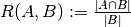
confusion_matrix 函数通过计算 confusion matrix(混淆矩阵) 来 evaluates classification accuracy (评估分类的准确性)。
根据定义,confusion matrix (混淆矩阵)中的 entry(条目)  ,是实际上在 group 中的 observations (观察数),但预测在 group
  中。这里是一个示例:
>>> from sklearn.metrics import confusion_matrix
>>> y_true = [2, 0, 2, 2, 0, 1]
>>> y_pred = [0, 0, 2, 2, 0, 2]
>>> confusion_matrix(y_true, y_pred)
array([[2, 0, 0],
 [0, 0, 1],
 [1, 0, 2]])
这是一个这样的 confusion matrix (混淆矩阵)的可视化表示 (这个数字来自于 Confusion matrix):

对于 binary problems (二分类问题),我们可以得到 true negatives(真 negatives), false positives(假 positives), false negatives(假 negatives) 和 true positives(真 positives) 的数量如下:
>>> y_true = [0, 0, 0, 1, 1, 1, 1, 1]
>>> y_pred = [0, 1, 0, 1, 0, 1, 0, 1]
>>> tn, fp, fn, tp = confusion_matrix(y_true, y_pred).ravel()
>>> tn, fp, fn, tp
(2, 1, 2, 3)
示例:
- 参阅 Confusion matrix 例如使用 confusion matrix (混淆矩阵)来评估 classifier (分类器)的输出质量。
- 参阅 Recognizing hand-written digits 例如使用 confusion matrix (混淆矩阵)来分类手写数字。
- 参阅 Classification of text documents using sparse features 例如使用 confusion matrix (混淆矩阵)对文本文档进行分类。
3.3.2.5. 分类报告
classification_report 函数构建一个显示 main classification metrics (主分类指标)的文本报告。这是一个小例子,其中包含自定义的 target_names 和 inferred labels (推断标签):
>>> from sklearn.metrics import classification_report
>>> y_true = [0, 1, 2, 2, 0]
>>> y_pred = [0, 0, 2, 1, 0]
>>> target_names = ['class 0', 'class 1', 'class 2']
>>> print(classification_report(y_true, y_pred, target_names=target_names))
 precision    recall  f1-score   support

 class 0       0.67      1.00      0.80         2
 class 1       0.00      0.00      0.00         1
 class 2       1.00      0.50      0.67         2

avg / total       0.67      0.60      0.59         5
示例:
- 参阅 Recognizing hand-written digits 作为手写数字的分类报告的使用示例。
- 参阅 Classification of text documents using sparse features 作为文本文档的分类报告使用的示例。
- 参阅 Parameter estimation using grid search with cross-validation 例如使用 grid search with nested cross-validation (嵌套交叉验证进行网格搜索)的分类报告。
3.3.2.6. 汉明损失
hamming_loss 计算两组样本之间的 average Hamming loss (平均汉明损失)或者 Hamming distance(汉明距离) 。
如果  是给定样本的第 个标签的预测值,则
  是相应的真实值,而
  是 classes or labels (类或者标签)的数量,则两个样本之间的 Hamming loss (汉明损失)
  定义为:
定义为:
其中 是 indicator function(指标函数).
>>> from sklearn.metrics import hamming_loss
>>> y_pred = [1, 2, 3, 4]
>>> y_true = [2, 2, 3, 4]
>>> hamming_loss(y_true, y_pred)
0.25
在具有 binary label indicators (二分标签指示符)的 multilabel (多标签)情况下:
>>> hamming_loss(np.array([[0, 1], [1, 1]]), np.zeros((2, 2)))
0.75
Note
在 multiclass classification (多类分类)中, Hamming loss (汉明损失)对应于 y_true 和 y_pred 之间的 Hamming distance(汉明距离),它类似于 零一损失 函数。然而, zero-one loss penalizes (0-1损失惩罚)不严格匹配真实集合的预测集,Hamming loss (汉明损失)惩罚 individual labels (独立标签)。因此,Hamming loss(汉明损失)高于 zero-one loss(0-1 损失),总是在 0 和 1 之间,包括 0 和 1;预测真正的标签的正确的 subset or superset (子集或超集)将给出 0 和 1 之间的 Hamming loss(汉明损失)。
3.3.2.7. Jaccard 相似系数 score
jaccard_similarity_score 函数计算 pairs of label sets (标签组对)之间的 Jaccard similarity coefficients 也称作 Jaccard index 的平均值(默认)或总和。
将第 个样本的 Jaccard similarity coefficient 与 被标注过的真实数据的标签集 和 predicted label set (预测标签集):math:<cite>hat{y}_i</cite> 定义为
在 binary and multiclass classification (二分和多类分类)中,Jaccard similarity coefficient score 等于 classification accuracy(分类精度)。
>>> import numpy as np
>>> from sklearn.metrics import jaccard_similarity_score
>>> y_pred = [0, 2, 1, 3]
>>> y_true = [0, 1, 2, 3]
>>> jaccard_similarity_score(y_true, y_pred)
0.5
>>> jaccard_similarity_score(y_true, y_pred, normalize=False)
2
在具有 binary label indicators (二分标签指示符)的 multilabel (多标签)情况下:
>>> jaccard_similarity_score(np.array([[0, 1], [1, 1]]), np.ones((2, 2)))
0.75
3.3.2.8. 精准,召回和 F-measures
直观地来理解,precision 是 the ability of the classifier not to label as positive a sample that is negative (classifier (分类器)的标签不能被标记为正的样本为负的能力),并且 recall 是 classifier (分类器)查找所有 positive samples (正样本)的能力。
F-measure ( 和
和  measures) 可以解释为 precision (精度)和 recall (召回)的 weighted harmonic mean (加权调和平均值)。 measure 值达到其最佳值 1 ,其最差分数为 0 。与
  , 和 是等价的, recall (召回)和 precision (精度)同样重要。
precision_recall_curve 通过改变 decision threshold (决策阈值)从 ground truth label (被标记的真实数据标签) 和 score given by the classifier (分类器给出的分数)计算 precision-recall curve (精确召回曲线)。
average_precision_score 函数根据 prediction scores (预测分数)计算出 average precision (AP)(平均精度)。该分数对应于 precision-recall curve (精确召回曲线)下的面积。该值在 0 和 1 之间,并且越高越好。通过 random predictions (随机预测), AP 是 fraction of positive samples (正样本的分数)。
几个函数可以让您 analyze the precision (分析精度),recall(召回) 和 F-measures 得分:
| average_precision_score(y_true, y_score[, …]) | Compute average precision (AP) from prediction scores | | f1_score(y_true, y_pred[, labels, …]) | Compute the F1 score, also known as balanced F-score or F-measure | | fbeta_score(y_true, y_pred, beta[, labels, …]) | Compute the F-beta score | | precision_recall_curve(y_true, probas_pred) | Compute precision-recall pairs for different probability thresholds | | precision_recall_fscore_support(y_true, y_pred) | Compute precision, recall, F-measure and support for each class | | precision_score(y_true, y_pred[, labels, …]) | Compute the precision | | recall_score(y_true, y_pred[, labels, …]) | Compute the recall |
请注意,precision_recall_curve 函数仅限于 binary case (二分情况)。 average_precision_score 函数只适用于 binary classification and multilabel indicator format (二分类和多标签指示器格式)。
示例:
- 参阅 Classification of text documents using sparse features 例如
f1_score用于分类文本文档的用法。 - 参阅 Parameter estimation using grid search with cross-validation 例如
precision_score和recall_score用于 using grid search with nested cross-validation (使用嵌套交叉验证的网格搜索)来估计参数。 - 参阅 Precision-Recall 例如
precision_recall_curve用于 evaluate classifier output quality(评估分类器输出质量)。
3.3.2.8.1. 二分类
在二分类任务中,术语 ‘’positive(正)’’ 和 ‘’negative(负)’’ 是指 classifier’s prediction (分类器的预测),术语 ‘’true(真)’’ 和 ‘’false(假)’’ 是指该预测是否对应于 external judgment (外部判断)(有时被称为 ‘’observation(观测值)’‘)。给出这些定义,我们可以指定下表:
| | Actual class (observation) | | Predicted class (expectation) | tp (true positive) Correct result | fp (false positive) Unexpected result | | fn (false negative) Missing result | tn (true negative) Correct absence of result |
在这种情况下,我们可以定义 precision(精度), recall(召回) 和 F-measure 的概念:
以下是 binary classification (二分类)中的一些小例子:
>>> from sklearn import metrics
>>> y_pred = [0, 1, 0, 0]
>>> y_true = [0, 1, 0, 1]
>>> metrics.precision_score(y_true, y_pred)
1.0
>>> metrics.recall_score(y_true, y_pred)
0.5
>>> metrics.f1_score(y_true, y_pred)
0.66...
>>> metrics.fbeta_score(y_true, y_pred, beta=0.5)
0.83...
>>> metrics.fbeta_score(y_true, y_pred, beta=1)
0.66...
>>> metrics.fbeta_score(y_true, y_pred, beta=2)
0.55...
>>> metrics.precision_recall_fscore_support(y_true, y_pred, beta=0.5)
(array([ 0.66...,  1\.        ]), array([ 1\. ,  0.5]), array([ 0.71...,  0.83...]), array([2, 2]...))

>>> import numpy as np
>>> from sklearn.metrics import precision_recall_curve
>>> from sklearn.metrics import average_precision_score
>>> y_true = np.array([0, 0, 1, 1])
>>> y_scores = np.array([0.1, 0.4, 0.35, 0.8])
>>> precision, recall, threshold = precision_recall_curve(y_true, y_scores)
>>> precision
array([ 0.66...,  0.5       ,  1\.        ,  1\.        ])
>>> recall
array([ 1\. ,  0.5,  0.5,  0\. ])
>>> threshold
array([ 0.35,  0.4 ,  0.8 ])
>>> average_precision_score(y_true, y_scores)
0.83...
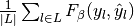
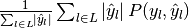
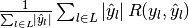
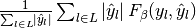
3.3.2.8.2. 多类和多标签分类
在 multiclass and multilabel classification task(多类和多标签分类任务)中,precision(精度), recall(召回), and F-measures 的概念可以独立地应用于每个标签。 有以下几种方法 combine results across labels (将结果跨越标签组合),由 average 参数指定为 average_precision_score (仅用于 multilabel), f1_score, fbeta_score, precision_recall_fscore_support, precision_score 和 recall_score 函数,如上 above 所述。请注意,对于在包含所有标签的多类设置中进行 “micro”-averaging (”微”平均),将产生相等的 precision(精度), recall(召回)和  ,而 “weighted(加权)” averaging(平均)可能会产生 precision(精度)和 recall(召回)之间的 F-score 。
为了使这一点更加明确,请考虑以下 notation (符号):
 predicted(预测)
  对
对 true(真) 对
 labels 集合
 samples 集合
 的子集与样本
  , 即
, 即 
 的子集与 label
- 类似的,
 和
和  是 的子集
是 的子集 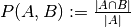
 (Conventions (公约)在处理
  有所不同; 这个实现使用
  , 与
, 与  类似.)
类似.)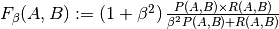
然后将 metrics (指标)定义为:
average |
Precision | Recall | F_beta |
|---|---|---|---|
"micro" |
 |
 |
 |
"samples" |
 |
 |
 |
"macro" |
 |
 |
 |
"weighted" |
 |
 |
 |
None |
 |
 |
 |
>>> from sklearn import metrics
>>> y_true = [0, 1, 2, 0, 1, 2]
>>> y_pred = [0, 2, 1, 0, 0, 1]
>>> metrics.precision_score(y_true, y_pred, average='macro')
0.22...
>>> metrics.recall_score(y_true, y_pred, average='micro')
...
0.33...
>>> metrics.f1_score(y_true, y_pred, average='weighted')
0.26...
>>> metrics.fbeta_score(y_true, y_pred, average='macro', beta=0.5)
0.23...
>>> metrics.precision_recall_fscore_support(y_true, y_pred, beta=0.5, average=None)
...
(array([ 0.66...,  0\.        ,  0\.        ]), array([ 1.,  0.,  0.]), array([ 0.71...,  0\.        ,  0\.        ]), array([2, 2, 2]...))
For multiclass classification with a “negative class”, it is possible to exclude some labels:
>>> metrics.recall_score(y_true, y_pred, labels=[1, 2], average='micro')
... # excluding 0, no labels were correctly recalled
0.0
Similarly, labels not present in the data sample may be accounted for in macro-averaging.
>>> metrics.precision_score(y_true, y_pred, labels=[0, 1, 2, 3], average='macro')
...
0.166...
3.3.2.9. Hinge loss
hinge_loss 函数使用 hinge loss 计算模型和数据之间的 average distance (平均距离),这是一种只考虑 prediction errors (预测误差)的 one-sided metric (单向指标)。(Hinge loss 用于最大边界分类器,如支持向量机)
如果标签用 +1 和 -1 编码,则 : 是真实值,并且  是由
是由 decision_function 输出的 predicted decisions (预测决策),则 hinge loss 定义为:

如果有两个以上的标签, hinge_loss 由于 Crammer & Singer 而使用了 multiclass variant (多类型变体)。 Here 是描述它的论文。
如果  是真实标签的 predicted decision (预测决策),并且
  是所有其他标签的预测决策的最大值,其中预测决策由 decision function (决策函数)输出,则 multiclass hinge loss 定义如下:

这里是一个小例子,演示了在 binary class (二类)问题中使用了具有 svm classifier (svm 的分类器)的 hinge_loss 函数:
>>> from sklearn import svm
>>> from sklearn.metrics import hinge_loss
>>> X = [[0], [1]]
>>> y = [-1, 1]
>>> est = svm.LinearSVC(random_state=0)
>>> est.fit(X, y)
LinearSVC(C=1.0, class_weight=None, dual=True, fit_intercept=True,
 intercept_scaling=1, loss='squared_hinge', max_iter=1000,
 multi_class='ovr', penalty='l2', random_state=0, tol=0.0001,
 verbose=0)
>>> pred_decision = est.decision_function([[-2], [3], [0.5]])
>>> pred_decision
array([-2.18...,  2.36...,  0.09...])
>>> hinge_loss([-1, 1, 1], pred_decision)
0.3...
这里是一个示例,演示了在 multiclass problem (多类问题)中使用了具有 svm 分类器的 hinge_loss 函数:
>>> X = np.array([[0], [1], [2], [3]])
>>> Y = np.array([0, 1, 2, 3])
>>> labels = np.array([0, 1, 2, 3])
>>> est = svm.LinearSVC()
>>> est.fit(X, Y)
LinearSVC(C=1.0, class_weight=None, dual=True, fit_intercept=True,
 intercept_scaling=1, loss='squared_hinge', max_iter=1000,
 multi_class='ovr', penalty='l2', random_state=None, tol=0.0001,
 verbose=0)
>>> pred_decision = est.decision_function([[-1], [2], [3]])
>>> y_true = [0, 2, 3]
>>> hinge_loss(y_true, pred_decision, labels)
0.56...
3.3.2.10. Log 损失
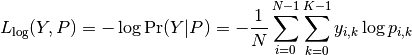
Log loss,又被称为 logistic regression loss(logistic 回归损失)或者 cross-entropy loss(交叉熵损失) 定义在 probability estimates (概率估计)。它通常用于 (multinomial) logistic regression ((多项式)logistic 回归)和 neural networks (神经网络)以及 expectation-maximization (期望最大化)的一些变体中,并且可用于评估分类器的 probability outputs (概率输出)(predict_proba)而不是其 discrete predictions (离散预测)。
对于具有真实标签  的 binary classification (二分类)和 probability estimate (概率估计)
  , 每个样本的 log loss 是给定的分类器的 negative log-likelihood 真正的标签:

这扩展到 multiclass case (多类案例)如下。 让一组样本的真实标签被编码为 1-of-K binary indicator matrix  , 即 如果样本 具有取自一组
  个标签的标签
  ,则
,则  。令 为 matrix of probability estimates (概率估计矩阵),
 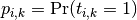 。那么整套的 log loss 就是
为了看这这里如何 generalizes (推广)上面给出的 binary log loss (二分 log loss),请注意,在 binary case (二分情况下), 和
和 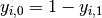 ,因此扩展
,因此扩展  的 inner sum (内部和),给出 binary log loss (二分 log loss)。
log_loss 函数计算出一个 a list of ground-truth labels (已标注的真实数据的标签的列表)和一个 probability matrix (概率矩阵) 的 log loss,由 estimator (估计器)的 predict_proba 方法返回。
>>> from sklearn.metrics import log_loss
>>> y_true = [0, 0, 1, 1]
>>> y_pred = [[.9, .1], [.8, .2], [.3, .7], [.01, .99]]
>>> log_loss(y_true, y_pred)
0.1738...
y_pred 中的第一个 [.9, .1] 表示第一个样本具有标签 0 的 90% 概率。log loss 是非负数。
3.3.2.11. 马修斯相关系数
matthews_corrcoef 函数用于计算 binary classes (二分类)的 Matthew’s correlation coefficient (MCC) 引用自 Wikipedia:
“Matthews correlation coefficient(马修斯相关系数)用于机器学习,作为 binary (two-class) classifications (二分类)分类质量的度量。它考虑到 true and false positives and negatives (真和假的 positives 和 negatives),通常被认为是可以使用的 balanced measure(平衡措施),即使 classes are of very different sizes (类别大小不同)。MCC 本质上是 -1 和 +1 之间的相关系数值。系数 +1 表示完美预测,0 表示平均随机预测, -1 表示反向预测。statistic (统计量)也称为 phi coefficient (phi)系数。”
在 binary (two-class) (二分类)情况下, ,
,  ,
,  和
和  分别是 true positives, true negatives, false positives 和 false negatives 的数量,MCC 定义为
在 multiclass case (多类的情况)下, Matthews correlation coefficient(马修斯相关系数) 可以根据 classes (类)的 confusion_matrix  定义 defined 。为了简化定义,考虑以下中间变量:
 真正发生了 类的次数,
 类被预测的次数,
 正确预测的样本总数,
 样本总数.
样本总数.
然后 multiclass MCC 定义为:

当有两个以上的标签时, MCC 的值将不再在 -1 和 +1 之间。相反,根据已经标注的真实数据的数量和分布情况,最小值将介于 -1 和 0 之间。最大值始终为 +1 。
这是一个小例子,说明了使用 matthews_corrcoef 函数:
>>> from sklearn.metrics import matthews_corrcoef
>>> y_true = [+1, +1, +1, -1]
>>> y_pred = [+1, -1, +1, +1]
>>> matthews_corrcoef(y_true, y_pred)
-0.33...
3.3.2.12. Receiver operating characteristic (ROC)
函数 roc_curve 计算 receiver operating characteristic curve, or ROC curve. 引用 Wikipedia :
“A receiver operating characteristic (ROC), 或者简单的 ROC 曲线,是一个图形图,说明了 binary classifier (二分分类器)系统的性能,因为 discrimination threshold (鉴别阈值)是变化的。它是通过在不同的阈值设置下,从 true positives out of the positives (TPR = true positive 比例) 与 false positives out of the negatives (FPR = false positive 比例) 绘制 true positive 的比例来创建的。 TPR 也称为 sensitivity(灵敏度),FPR 是减去 specificity(特异性) 或 true negative 比例。”
该函数需要真正的 binar value (二分值)和 target scores(目标分数),这可以是 positive class 的 probability estimates (概率估计),confidence values(置信度值)或 binary decisions(二分决策)。 这是一个如何使用 roc_curve 函数的小例子:
>>> import numpy as np
>>> from sklearn.metrics import roc_curve
>>> y = np.array([1, 1, 2, 2])
>>> scores = np.array([0.1, 0.4, 0.35, 0.8])
>>> fpr, tpr, thresholds = roc_curve(y, scores, pos_label=2)
>>> fpr
array([ 0\. ,  0.5,  0.5,  1\. ])
>>> tpr
array([ 0.5,  0.5,  1\. ,  1\. ])
>>> thresholds
array([ 0.8 ,  0.4 ,  0.35,  0.1 ])
该图显示了这样的 ROC 曲线的示例:

roc_auc_score 函数计算 receiver operating characteristic (ROC) 曲线下的面积,也由 AUC 和 AUROC 表示。通过计算 roc 曲线下的面积,曲线信息总结为一个数字。 有关更多的信息,请参阅 Wikipedia article on AUC .
>>> import numpy as np
>>> from sklearn.metrics import roc_auc_score
>>> y_true = np.array([0, 0, 1, 1])
>>> y_scores = np.array([0.1, 0.4, 0.35, 0.8])
>>> roc_auc_score(y_true, y_scores)
0.75
在 multi-label classification (多标签分类)中, roc_auc_score 函数通过在标签上进行平均来扩展 above .
与诸如 subset accuracy (子集精确度),Hamming loss(汉明损失)或 F1 score 的 metrics(指标)相比, ROC 不需要优化每个标签的阈值。roc_auc_score 函数也可以用于 multi-class classification (多类分类),如果预测的输出被 binarized (二分化)。

示例:
- 参阅 Receiver Operating Characteristic (ROC) 例如使用 ROC 来评估分类器输出的质量。
- 参阅 Receiver Operating Characteristic (ROC) with cross validation 例如使用 ROC 来评估分类器输出质量,使用 cross-validation (交叉验证)。
- 参阅 Species distribution modeling 例如使用 ROC 来 model species distribution 模拟物种分布。
3.3.2.13. 零一损失
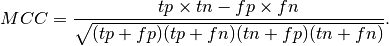
zero_one_loss 函数通过  计算 0-1 classification loss (
 ) 的 sum (和)或 average (平均值)。默认情况下,函数在样本上 normalizes (标准化)。要获得 的总和,将
 normalize 设置为 False。
在 multilabel classification (多标签分类)中,如果零标签与标签严格匹配,则 zero_one_loss 将一个子集作为一个子集,如果有任何错误,则为零。默认情况下,函数返回不完全预测子集的百分比。为了得到这样的子集的计数,将 normalize 设置为 False 。
如果 是第 个样本的预测值, 是相应的真实值,则 0-1 loss 定义为:

其中 是 indicator function.
>>> from sklearn.metrics import zero_one_loss
>>> y_pred = [1, 2, 3, 4]
>>> y_true = [2, 2, 3, 4]
>>> zero_one_loss(y_true, y_pred)
0.25
>>> zero_one_loss(y_true, y_pred, normalize=False)
1
在具有 binary label indicators (二分标签指示符)的 multilabel (多标签)情况下,第一个标签集 [0,1] 有错误:
>>> zero_one_loss(np.array([[0, 1], [1, 1]]), np.ones((2, 2)))
0.5

>>> zero_one_loss(np.array([[0, 1], [1, 1]]), np.ones((2, 2)),  normalize=False)
1
示例:
- 参阅 Recursive feature elimination with cross-validation 例如 zero one loss 使用以通过 cross-validation (交叉验证)执行递归特征消除。
3.3.2.14. Brier 分数损失
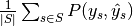
brier_score_loss 函数计算二进制类的 Brier 分数 。引用维基百科:
“Brier 分数是一个特有的分数函数,用于衡量概率预测的准确性。它适用于预测必须将概率分配给一组相互排斥的离散结果的任务。”
该函数返回的是 实际结果与可能结果 的预测概率之间均方差的得分。 实际结果必须为1或0(真或假),而实际结果的预测概率可以是0到1之间的值。
Brier 分数损失也在0到1之间,分数越低(均方差越小),预测越准确。它可以被认为是对一组概率预测的 “校准” 的度量。
其中:  是预测的总数,
  是实际结果
是实际结果  的预测概率。
这是一个使用这个函数的小例子:
>>> import numpy as np
>>> from sklearn.metrics import brier_score_loss
>>> y_true = np.array([0, 1, 1, 0])
>>> y_true_categorical = np.array(["spam", "ham", "ham", "spam"])
>>> y_prob = np.array([0.1, 0.9, 0.8, 0.4])
>>> y_pred = np.array([0, 1, 1, 0])
>>> brier_score_loss(y_true, y_prob)
0.055
>>> brier_score_loss(y_true, 1-y_prob, pos_label=0)
0.055
>>> brier_score_loss(y_true_categorical, y_prob, pos_label="ham")
0.055
>>> brier_score_loss(y_true, y_prob > 0.5)
0.0
示例:
- 请参阅分类器的概率校准 Probability calibration of classifiers ,通过 Brier 分数损失使用示例 来执行分类器的概率校准。
参考文献:
-
- Brier, 以概率表示的预测验证 , 月度天气评估78.1(1950)
3.3.3. 多标签排名指标
在多分类学习中,每个样本可以具有与其相关联的任何数量的真实标签。目标是给予高分,更好地评价真实标签。
3.3.3.1. 覆盖误差
coverage_error 函数计算必须包含在最终预测中的标签的平均数,以便预测所有真正的标签。 如果您想知道有多少 top 评分标签,您必须通过平均来预测,而不会丢失任何真正的标签,这很有用。 因此,此指标的最佳价值是真正标签的平均数量。
Note
我们的实现的分数比 Tsoumakas 等人在2010年的分数大1。 这扩展了它来处理一个具有0个真实标签实例的退化情况。
正式地,给定真实标签  的二进制指示矩阵和与每个标签
  相关联的分数,覆盖范围被定义为

与  。给定等级定义,通过给出将被分配给所有绑定值的最大等级,
 y_scores 中的关系会被破坏。
这是一个使用这个函数的小例子:
>>> import numpy as np
>>> from sklearn.metrics import coverage_error
>>> y_true = np.array([[1, 0, 0], [0, 0, 1]])
>>> y_score = np.array([[0.75, 0.5, 1], [1, 0.2, 0.1]])
>>> coverage_error(y_true, y_score)
2.5
3.3.3.2. 标签排名平均精度
label_ranking_average_precision_score 函数实现标签排名平均精度(LRAP)。 该度量值与 average_precision_score 函数相关联,但是基于标签排名的概念,而不是精确度和召回。
标签排名平均精度(LRAP)是分配给每个样本的每个真实标签的平均值,真实对总标签与较低分数的比率。 如果能够为每个样本相关标签提供更好的排名,这个指标就会产生更好的分数。 获得的得分总是严格大于0,最佳值为1。如果每个样本只有一个相关标签,则标签排名平均精度等于 平均倒数等级 。
正式地,给定真实标签  的二进制指示矩阵和与每个标签
  相关联的得分,平均精度被定义为

与  , 和
, 和  是集合的 l0 范数或基数。
这是一个使用这个函数的小例子:
>>> import numpy as np
>>> from sklearn.metrics import label_ranking_average_precision_score
>>> y_true = np.array([[1, 0, 0], [0, 0, 1]])
>>> y_score = np.array([[0.75, 0.5, 1], [1, 0.2, 0.1]])
>>> label_ranking_average_precision_score(y_true, y_score)
0.416...
3.3.3.3. 排序损失
label_ranking_loss 函数计算在样本上平均排序错误的标签对数量的排序损失,即真实标签的分数低于假标签,由虚假和真实标签的倒数加权。最低可实现的排名损失为零。
正式地,给定真相标签 的二进制指示矩阵和与每个标签 相关联的得分,排序损失被定义为

其中 是  范数或集合的基数。
这是一个使用这个函数的小例子:
>>> import numpy as np
>>> from sklearn.metrics import label_ranking_loss
>>> y_true = np.array([[1, 0, 0], [0, 0, 1]])
>>> y_score = np.array([[0.75, 0.5, 1], [1, 0.2, 0.1]])
>>> label_ranking_loss(y_true, y_score)
0.75...
>>> # With the following prediction, we have perfect and minimal loss
>>> y_score = np.array([[1.0, 0.1, 0.2], [0.1, 0.2, 0.9]])
>>> label_ranking_loss(y_true, y_score)
0.0
参考文献:
- Tsoumakas, G., Katakis, I., & Vlahavas, I. (2010). 挖掘多标签数据。在数据挖掘和知识发现手册(第667-685页)。美国 Springer.
3.3.4. 回归指标
该 sklearn.metrics 模块实现了一些 loss, score 以及 utility 函数以测量 regression(回归)的性能. 其中一些已经被加强以处理多个输出的场景: mean_squared_error, mean_absolute_error, explained_variance_score 和 r2_score.
这些函数有 multioutput 这样一个 keyword(关键的)参数, 它指定每一个目标的 score(得分)或 loss(损失)的平均值的方式. 默认是 'uniform_average', 其指定了输出时一致的权重均值. 如果一个 ndarray 的 shape (n_outputs,) 被传递, 则其中的 entries(条目)将被解释为权重,并返回相应的加权平均值. 如果 multioutput 指定了 'raw_values' , 则所有未改变的部分 score(得分)或 loss(损失)将以 (n_outputs,) 形式的数组返回.
该 r2_score 和 explained_variance_score 函数接受一个额外的值 'variance_weighted' 用于 multioutput 参数. 该选项通过相应目标变量的方差使得每个单独的 score 进行加权. 该设置量化了全局捕获的未缩放方差. 如果目标变量的大小不一样, 则该 score 更好地解释了较高的方差变量. multioutput='variance_weighted' 是 r2_score 的默认值以向后兼容. 以后该值会被改成 uniform_average.
3.3.4.1. 解释方差得分
该 explained_variance_score 函数计算了 explained variance regression score(解释的方差回归得分).
如果 是预估的目标输出, 是相应(正确的)目标输出, 并且  is 方差, 标准差的平方, 那么解释的方差预估如下:
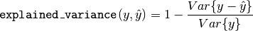
最好的得分是 1.0, 值越低越差.
下面是一下有关 explained_variance_score 函数使用的一些例子:
>>> from sklearn.metrics import explained_variance_score
>>> y_true = [3, -0.5, 2, 7]
>>> y_pred = [2.5, 0.0, 2, 8]
>>> explained_variance_score(y_true, y_pred)
0.957...
>>> y_true = [[0.5, 1], [-1, 1], [7, -6]]
>>> y_pred = [[0, 2], [-1, 2], [8, -5]]
>>> explained_variance_score(y_true, y_pred, multioutput='raw_values')
...
array([ 0.967...,  1\.        ])
>>> explained_variance_score(y_true, y_pred, multioutput=[0.3, 0.7])
...
0.990...
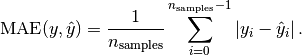
3.3.4.2. 平均绝对误差
该 mean_absolute_error 函数计算了 平均绝对误差, 一个对应绝对误差损失预期值或者  -norm 损失的风险度量.
如果 是 -th 样本的预测值, 并且 是对应的真实值, 则平均绝对误差 (MAE) 预估的 定义如下
下面是一个有关 mean_absolute_error 函数用法的小例子:
>>> from sklearn.metrics import mean_absolute_error
>>> y_true = [3, -0.5, 2, 7]
>>> y_pred = [2.5, 0.0, 2, 8]
>>> mean_absolute_error(y_true, y_pred)
0.5
>>> y_true = [[0.5, 1], [-1, 1], [7, -6]]
>>> y_pred = [[0, 2], [-1, 2], [8, -5]]
>>> mean_absolute_error(y_true, y_pred)
0.75
>>> mean_absolute_error(y_true, y_pred, multioutput='raw_values')
array([ 0.5,  1\. ])
>>> mean_absolute_error(y_true, y_pred, multioutput=[0.3, 0.7])
...
0.849...
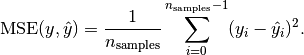
3.3.4.3. 均方误差
该 mean_squared_error 函数计算了 均方误差, 一个对应于平方(二次)误差或损失的预期值的风险度量.
如果 是 -th 样本的预测值, 并且 是对应的真实值, 则均方误差(MSE)预估的 定义如下
下面是一个有关 mean_squared_error 函数用法的小例子:
>>> from sklearn.metrics import mean_squared_error
>>> y_true = [3, -0.5, 2, 7]
>>> y_pred = [2.5, 0.0, 2, 8]
>>> mean_squared_error(y_true, y_pred)
0.375
>>> y_true = [[0.5, 1], [-1, 1], [7, -6]]
>>> y_pred = [[0, 2], [-1, 2], [8, -5]]
>>> mean_squared_error(y_true, y_pred)
0.7083...
Examples:
- 点击 Gradient Boosting regression 查看均方误差用于梯度上升(gradient boosting)回归的使用例子。
3.3.4.4. 均方误差对数
该 mean_squared_log_error 函数计算了一个对应平方对数(二次)误差或损失的预估值风险度量.
如果 是 -th 样本的预测值, 并且 是对应的真实值, 则均方误差对数(MSLE)预估的 定义如下
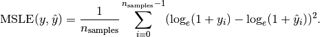
其中  表示
表示  的自然对数. 当目标具有指数增长的趋势时, 该指标最适合使用, 例如人口数量, 跨年度商品的平均销售额等. 请注意, 该指标会对低于预测的估计值进行估计.
下面是一个有关 mean_squared_log_error 函数用法的小例子:
>>> from sklearn.metrics import mean_squared_log_error
>>> y_true = [3, 5, 2.5, 7]
>>> y_pred = [2.5, 5, 4, 8]
>>> mean_squared_log_error(y_true, y_pred)
0.039...
>>> y_true = [[0.5, 1], [1, 2], [7, 6]]
>>> y_pred = [[0.5, 2], [1, 2.5], [8, 8]]
>>> mean_squared_log_error(y_true, y_pred)
0.044...
3.3.4.5. 中位绝对误差
该 median_absolute_error 函数尤其有趣, 因为它的离群值很强. 通过取目标和预测之间的所有绝对差值的中值来计算损失.
如果 是 -th 样本的预测值, 并且 是对应的真实值, 则中位绝对误差(MedAE)预估的 定义如下

该 median_absolute_error 函数不支持多输出.
下面是一个有关 median_absolute_error 函数用法的小例子:
>>> from sklearn.metrics import median_absolute_error
>>> y_true = [3, -0.5, 2, 7]
>>> y_pred = [2.5, 0.0, 2, 8]
>>> median_absolute_error(y_true, y_pred)
0.5
3.3.4.6. R² score, 可决系数
该 r2_score 函数计算了 computes R², 即 可决系数. 它提供了将来样本如何可能被模型预测的估量. 最佳分数为 1.0, 可以为负数(因为模型可能会更糟). 总是预测 y 的预期值,不考虑输入特征的常数模型将得到 R^2 得分为 0.0.
如果 是 -th 样本的预测值, 并且 是对应的真实值, 则 R² 得分预估的 定义如下
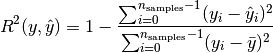
其中 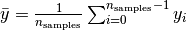 .
.
下面是一个有关 r2_score 函数用法的小例子:
>>> from sklearn.metrics import r2_score
>>> y_true = [3, -0.5, 2, 7]
>>> y_pred = [2.5, 0.0, 2, 8]
>>> r2_score(y_true, y_pred)
0.948...
>>> y_true = [[0.5, 1], [-1, 1], [7, -6]]
>>> y_pred = [[0, 2], [-1, 2], [8, -5]]
>>> r2_score(y_true, y_pred, multioutput='variance_weighted')
...
0.938...
>>> y_true = [[0.5, 1], [-1, 1], [7, -6]]
>>> y_pred = [[0, 2], [-1, 2], [8, -5]]
>>> r2_score(y_true, y_pred, multioutput='uniform_average')
...
0.936...
>>> r2_score(y_true, y_pred, multioutput='raw_values')
...
array([ 0.965...,  0.908...])
>>> r2_score(y_true, y_pred, multioutput=[0.3, 0.7])
...
0.925...
示例:
- 点击 Lasso and Elastic Net for Sparse Signals 查看关于R²用于评估在Lasso and Elastic Net on sparse signals上的使用.
3.3.5. 聚类指标
该 sklearn.metrics 模块实现了一些 loss, score 和 utility 函数. 更多信息请参阅 聚类性能度量 部分, 例如聚类, 以及用于二分聚类的 Biclustering 评测.
3.3.6. 虚拟估计
在进行监督学习的过程中,简单的 sanity check(理性检查)包括将人的估计与简单的经验法则进行比较. DummyClassifier 实现了几种简单的分类策略:
-
stratified通过在训练集类分布方面来生成随机预测. -
most_frequent总是预测训练集中最常见的标签. -
prioralways predicts the class that maximizes the class prior (likemost_frequent) and ``predict_proba` returns the class prior. -
uniform随机产生预测. -
constant 总是预测用户提供的常量标签.A major motivation of this method is F1-scoring, when the positive class is in the minority. 这种方法的主要动机是 F1-scoring, 当 positive class(正类)较少时.
请注意, 这些所有的策略, predict 方法彻底的忽略了输入数据!
为了说明 DummyClassifier, 首先让我们创建一个 imbalanced dataset:
>>> from sklearn.datasets import load_iris
>>> from sklearn.model_selection import train_test_split
>>> iris = load_iris()
>>> X, y = iris.data, iris.target
>>> y[y != 1] = -1
>>> X_train, X_test, y_train, y_test = train_test_split(X, y, random_state=0)
接下来, 让我们比较一下 SVC 和 most_frequent 的准确性.
>>> from sklearn.dummy import DummyClassifier
>>> from sklearn.svm import SVC
>>> clf = SVC(kernel='linear', C=1).fit(X_train, y_train)
>>> clf.score(X_test, y_test)
0.63...
>>> clf = DummyClassifier(strategy='most_frequent',random_state=0)
>>> clf.fit(X_train, y_train)
DummyClassifier(constant=None, random_state=0, strategy='most_frequent')
>>> clf.score(X_test, y_test)
0.57...
我们看到 SVC 没有比一个 dummy classifier(虚拟分类器)好很多. 现在, 让我们来更改一下 kernel:
>>> clf = SVC(kernel='rbf', C=1).fit(X_train, y_train)
>>> clf.score(X_test, y_test)
0.97...
我们看到准确率提升到将近 100%. 建议采用交叉验证策略, 以更好地估计精度, 如果不是太耗 CPU 的话. 更多信息请参阅 交叉验证:评估估算器的表现 部分. 此外,如果要优化参数空间,强烈建议您使用适当的方法; 更多详情请参阅 调整估计器的超参数 部分.
通常来说,当分类器的准确度太接近随机情况时,这可能意味着出现了一些问题: 特征没有帮助, 超参数没有正确调整, class 不平衡造成分类器有问题等…
DummyRegressor 还实现了四个简单的经验法则来进行回归:
mean总是预测训练目标的平均值.median总是预测训练目标的中位数.quantile总是预测用户提供的训练目标的 quantile(分位数).constant总是预测由用户提供的常数值.
在以上所有的策略中, predict 方法完全忽略了输入数据.